This page is a quote from the PhD Thesis of P. Brommer.

If there is a disadvantage to Powell's method as described above, it is that it readily jumps to the closest local minimum available, ignoring any other, perhaps even better local minima. As the sequence of $Z(\boldsymbol\xi_{i})$ is strictly monotonous, it is impossible to escape the attraction regime of a minimum. If this minimum does not happen to be the global optimum of the target function, the algorithm will not end up with the optimal solution. The Simulated Annealing method can be used to sample configuration space in search of the global minimum. It was first described by Kirkpatrick et al.¹ and is based on the work of Metropolis et al.².

The idea of Metropolis and coworkers is rather basic: When simulating an ensemble of atoms, a small random change is accepted, if the resulting change in energy $\Delta E,$ is negative. Changes with $\Delta E>0$ are accepted with a probability $P(\Delta E)=\exp(-\Delta E/k_{B}T)$ and rejected otherwise. Frequent application of this basic step is comparable to simulating the ensemble in a heat bath of temperature $T$. Due to the introduction of chance to the simulation, methods based on this idea are called Monte Carlo methods, as an allusion to the famous casino.

Kirkpatrick and coworkers now link statistical mechanics to the minimisation of a target function and apply the Metropolis rule to the latter problem. Starting from a state $\boldsymbol x$ a change by $\delta\boldsymbol x$ is accepted, if the target function $Z(\boldsymbol\xi)$ is improved by this step. Additionally, a change for the worse is accepted with a probability $P(\Delta Z)=\exp(-\Delta Z/T)$. $T$ is no longer a physical temperature, but an effective temperature in the units of the target function.

Analogous to annealing in metals, a system is first “heated” at a high effective temperature. Then $T$ is decreased slowly until the system “solidifies”. The temperature sequence is decisive: While quenching, i.e. a rapid decrease in temperature, will lead to trapping the target function in a local minimum (equivalent to a metastable state in a physical system), it is possible to attain the global minimum with a certain probability when cooling slowly enough.

Simulated annealing was first applied to discrete systems (e.g. the travelling salesman problem), where the “basic step”, which is either accepted or rejected, is clearly defined. In a system with continuous degrees of freedom like force matching, the basic step length has to be specified first. Corana et al.³ describe how this can be done adaptively. A step length vector $\boldsymbol v\in\mathbb{R}^n$ is defined, where the components are the typical step lengths in each coordinate direction of the configuration space. From a starting point $\boldsymbol x$ one generates a new point $\boldsymbol x'$ for one of the coordinate directions $h=1,\ldots,n$ with $$\boldsymbol{x}'=\boldsymbol{x}+rv_{h}\boldsymbol{e}_{h},$$ where $r$ is a (pseudo-)random number in $[-1,1]$ and $\boldsymbol e_{h}$ the $h^{\text{th}}$ coordinate unit vector. The Metropolis criterion is then applied to the $\boldsymbol x'$: A pseudorandom number $p'\in[0,1]$ is generated and the new $\boldsymbol x'$ is accepted if $p'<p=\exp(-\frac{Z(\boldsymbol{x}')-Z(\boldsymbol{x})}{T})$ and $\boldsymbol x:=\boldsymbol x'$. Then a trial point $\boldsymbol x'$ for the next coordinate direction is generated.

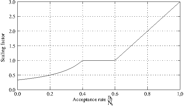
This is repeated $N_{s}$ times for each coordinate direction and the number of successful trials $n_{h}$ is recorded. That information is then used to adapt the step length $v_{h}$. The algorithm is most efficient, if approximately half of the suggested changes is accepted. A lower rejection rate implies that the steps are too small and too many function evaluations are needed to sample the configuration space. If the rejection rate is higher, much work is done in vain, because the steps are too big for the accessible configuration space. Corana and coworkers suggest changing $\boldsymbol v$ in the following way: $$v_{h} := v_{h} \left(1+2 \frac{n_{h}/N_{s}-0.6}{0.4}\right) \quad \text{if} n_{h}>0.6,N_{s},$$ $$v_{h} := \frac{v_{h}}{1+2 \frac{0.4-n_{h}/N_{s}}{0.4}} \quad\qquad\qquad \text{if} n_{h}<0.4,N_{s},$$ $$v_{h} := v_{h} \qquad\qquad\qquad\qquad\qquad\qquad\qquad\quad\text{else}.$$

This will modify the basic step length by a factor between 1/3 and 3. The step scaling function is plotted in Fig. 2.6.

Figure 2.6:The scaling factor for the basic MC step length depends on the acceptance rate. Both extremely high and extremely low rates are inefficient. From [4].

After $N_{T}$ step length adjustments, when the system is believed to have sampled the entire accessible configuration space, the effective temperature is reduced by a factor (e.g. $T'=0.85 T$), and the whole procedure is repeated at the lower temperature. Thus, the system is “cooled” slowly. Two conditions must be fulfilled to stop the algorithm:

1. Function values $Z(\boldsymbol x)$ at the end of consecutive temperature loops are close together, i.e. the system is trapped in a minimum.
2. The current function value is close to the optimal value $Z(x_{\text{opt}})$ reached so far.

If both criteria are met, $\boldsymbol x_{\text{opt}}$ is returned as a result. If only the first condition is fulfilled, the algorithm is stuck in a local minimum after visiting a better location. In this case, $\boldsymbol x$ is set to $\boldsymbol x_{\text{opt}}$ and the algorithm is continued from there.

Simulated Annealing is extremely expensive in function calls and thus in computation time, especially compared to Powell's method described above, but it has a chance of finding the global minimum, even if the starting point is not in the attraction regime. In [3], Corana et al. compare their algorithm to other optimisation procedures. They claim that although Simulated Annealing does need many function evaluations, it has the highest chance of obtaining the global minimum.

1. Kirkpatrick, S., Gelatt, C. D., and Vecci, M. P.: Optimization by simulated annealing. Science, 220 (4598), 671–680, 1983.
2. Metropolis, N., Rosenbluth, A., Rosenbluth, M., Teller, A., and Teller, E.: Equation of State Calculations by Fast Computing Machines. J. Chem. Phys., 21, 1087–1092, 1953.
3. Corana, A., Marchesi, M., Martini, C., and Ridella, S.: Minimizing Multimodal Functions of Continuous Variables with the “Simulated Annealing” Algorithm. ACM Trans. Math. Soft., 13 (3), 262–280, 1987.
4. Brommer, P.: Entwicklung und Test von Wechselwirkungspotenzialen in Quasikristallen. Master’s thesis, Universität Stuttgart, 2003.